30 Mart 2016 Çarşamba

Upsampling in Matlab


Here , we are going to use predesign matlab code for bilinear interpolation that i have been found from web. After that , we will call this matlab code in our upsampling program.Create that following code as bilinearInterpolation.m in your workplace that you will write upsampling program. They should be in the same directory.

function[out]=bilinearInterpolation(im,out_dims)
%// Get some necessary variables first
in_rows=size(im,1);
in_cols=size(im,2);
out_rows=out_dims(1);
out_cols=out_dims(2);

%// Lets S_R = R/R'
S_R = in_rows / out_rows;
%// Lets S_C = C/C'
S_C = in_cols / out_cols;

%// Define grid of co-ordinates in our image
%// Generate (x,y) pairs for each point in our image
[cf,rf]=meshgrid(1:out_cols,1:out_rows);

rf=rf*S_R;
cf=cf*S_C;

r=floor(rf);
c=floor(cf);

%// Any values out of range , cap
r(r<1)=1;
c(c<1)=1;
r(r>in_rows-1)=in_rows-1;
c(c>in_cols-1)=in_cols-1;

delta_R= rf-r;
delta_C=cf-c;

% Final line algorithm
%get column major indices for each point we wish to access

in1_ind= sub2ind([in_rows,in_cols],r,c);
in2_ind= sub2ind([in_rows,in_cols],r+1,c);
in3_ind= sub2ind([in_rows,in_cols],r,c+1);
in4_ind= sub2ind([in_rows,in_cols],r+1,c+1);

% now interpolate
% go through each channel for the case of colour
% create output image that is the same class as input

out=zeros(out_rows,out_cols,size(im,3));
out=cast(out,class(im));

for idx = 1:size(im,3)
chan=double(im(:,:,idx)); % get i th channel
% interpolate the channel
tmp=chan(in1_ind).*(1-delta_R).*(1-delta_C)+...
chan(in2_ind).*(delta_R).*(1-delta_C)+...
chan(in3_ind).*(1-delta_R).*(delta_C)+...
chan(in4_ind).*(delta_R).*(delta_C);
out(:,:,idx) = cast(tmp,class(im));
end


and finally following code is the upsampling matlab code , there is a scaled result of the image that i have chosen for my study called space elevator.


clear 
close all 
im=imread('SpaceElevator.jpg'); 
Rim = im(:,:,1); 
Gim = im(:,:,2); 
Bim = im(:,:,3); 

% Applying upsampling in levels 2,4 to our test image 
% Determine the dimensions of the source image 
[j k]=size(Rim); 
% Determine how much larger we want the new image(should be 
% an integer) 
scale=2; 
Rimup=bilinearInterpolation(Rim,[j*scale k*scale]); 
Gimup=bilinearInterpolation(Gim,[j*scale k*scale]); 
Bimup=bilinearInterpolation(Bim,[j*scale k*scale]); 
imup1=cat(3,Rimup,Gimup,Bimup); 

scale=4; 
Rimup=bilinearInterpolation(Rim,[j*scale k*scale]); 
Gimup=bilinearInterpolation(Gim,[j*scale k*scale]); 
Bimup=bilinearInterpolation(Bim,[j*scale k*scale]); 
imup2=cat(3,Rimup,Gimup,Bimup); 

figure(45); 
subplot(3,1,1);imagesc(im); 
subplot(3,1,2);imagesc(imup1); 
subplot(3,1,3);imagesc(imup2); 


29 Mart 2016 Salı

Lowpass and Bandpass filtering in spatial domain in Matlab

clear
close all
im1=imread('SpaceElevator.jpg');
figure(29);imshow(im1);
mask=[1 1 1; 1 1 1; 1 1 1]/9; % LOWPASS FILTER / MASKEMIZ
% Renk bilgisini kaybetmemek icin kırmızı,yeşil,mavi

% şeklinde üç adet dizi elde ediyoruz.
Rim = im1(:,:,1);
Gim = im1(:,:,2);
Bim = im1(:,:,3);

figure(32);imshow(Rim);
figure(33);imshow(Gim);
figure(34);imshow(Bim);

% her bir renk dizisini ayrı ayrı filtreliyoruz.
im4=uint8(conv2(mask,Rim,'full'));
im5=uint8(conv2(mask,Gim,'full'));
im6=uint8(conv2(mask,Bim,'full'));

figure(35);imshow(im4);
figure(36);imshow(im5);
figure(37);imshow(im6);

% cat fonksiyonu ile dosyayı geri elde ediyoruz.

image_RGB3=cat(3,im4,im5,im6);
figure(39);imshow(image_RGB3);

% BAND PASS SECTION
% Band geçiren filtre için 2 lowpass filtrenin farkını aldım.

mask2=[1 1 1;1 1 1;1 1 1]/25;
mask3=mask‐mask2;

% her bir renk dizisini ayrı ayrı filtreliyoruz.
im7=uint8(conv2(mask3,Rim,'full'));
im8=uint8(conv2(mask3,Gim,'full'));
im9=uint8(conv2(mask3,Bim,'full'));

figure(40);imshow(im7);
figure(41);imshow(im8);
figure(42);imshow(im9);

image_RGB4=cat(2,im7,im8,im9);
figure(43);imshow(image_RGB4);

image_RGB5=cat(3,im7,im8,im9);
figure(44);imshow(image_RGB5);

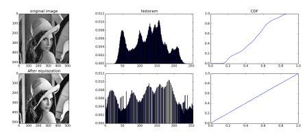
Histogram Equalization in Matlab

Histogram equalization is a method in image processing of contrast adjustment using the image's histogram.


% histogram equalization section 
J1=histeq(I3); 
J2=histeq(I4); 
J3=histeq(I5); 
J4=histeq(I6); 

% darkest image result 
figure(25) 
subplot(2,2,1); imshow(I3); 
subplot(2,2,2); imhist(I3); 
subplot(2,2,3); imshow(J1); 
subplot(2,2,4); imhist(J1); 

% dark image result 
figure(26) 
subplot(2,2,1); imshow(I4); 
subplot(2,2,2); imhist(I4); 
subplot(2,2,3); imshow(J2); 
subplot(2,2,4); imhist(J2); 

%light image result 
figure(27) 
subplot(2,2,1); imshow(I5); 
subplot(2,2,2); imhist(I5); 
subplot(2,2,3); imshow(J3); 
subplot(2,2,4); imhist(J3); 

%lightest image result 
figure(28) 
subplot(2,2,1); imshow(I6); 
subplot(2,2,2); imhist(I6); 
subplot(2,2,3); imshow(J4); 

subplot(2,2,4); imhist(J4); 

28 Mart 2016 Pazartesi

Bit Plane Slicing in Matlab

bit plane of a digital discrete signal (such as image or sound) is a set of bits corresponding to a given bit position in each of the binary numbers representing the signal.[1]
For example, for 16-bit data representation there are 16 bit planes: the first bit plane contains the set of the most significant bit, and the 16th contains the least significant bit.
It is possible to see that the first bit plane gives the roughest but the most critical approximation of values of a medium, and the higher the number of the bit plane, the less is its contribution to the final stage. Thus, adding a bit plane gives a better approximation.
If a bit on the nth bit plane on an m-bit dataset is set to 1, it contributes a value of 2(m-n), otherwise it contributes nothing. Therefore, bit planes can contribute half of the value of the previous bit plane. For example, in the 8-bit 10110101 (181 in decimal) the bit planes work as follows:


Bitplane is sometimes used as synonymous to Bitmap; however, technically the former refers to the location of the data in memory and the latter to the data itself.[2]
One aspect of using bit-planes is determining whether a bit-plane is random noise or contains significant information.
One method for calculating this is compare each pixel (X,Y) to three adjacent pixels (X-1,Y), (X,Y-1) and (X-1,Y-1). If the pixel is the same as at least two of the three adjacent pixels, it is not noise. A noisy bit-plane will have 49% to 51% pixels that are noise.[3]

Applications[edit]

As an example, in PCM sound encoding the first bit in the sample denotes the sign of the function, or in other words defines the half of the whole amplitude values range, and the last bit defines the precise value. Replacement of more significant bits result in more distortion than replacement of less significant bits. In lossy media compression that uses bit-planes it gives more freedom to encode less significant bit-planes and it is more critical to preserve the more significant ones.[4]
As illustrated in the image above, the early bitplanes, particularly the first, may have constant runs of bits, and thus can be efficiently encoded by run-length encoding. This is done (in the transform domain) in the Progressive Graphics File image format, for instance.
Some computers displayed graphics in bitplane format most notably the Amiga and Atari ST, contrasting with the more common packed format.

Programs[edit]

Many image processing packages can split an image into bit-planes. Open source tools such as Pamarith from Netpbm and Convert from ImageMagick can be used to generate bit-planes.


im=imread('SpaceElevator.jpg');      % imaj dosyasını okuma 
figure(7);imshow(im);                      % imaj dosyasının gösterimi 

I1 = rgb2gray(im);                            % resmi grayscale versiyona cevirme 
figure(8);imshow(I1); 

B1=bitget(I1,1); 
B1=B1*1;figure(9), imshow(logical(B1));title('Bit plane 1'); 
B2=bitget(I1,2); 
B2=B2*2;figure(10), imshow(logical(B2));title('Bit plane 2'); 
B3=bitget(I1,3); 
B3=B3*4;figure(11), imshow(logical(B3));title('Bit plane 3'); 
B4=bitget(I1,4); 
B4=B4*8;figure(12), imshow(logical(B4));title('Bit plane 4'); 
B5=bitget(I1,5); 
B5=B5*16;figure(13), imshow(logical(B5));title('Bit plane 5'); 
B6=bitget(I1,6); 
B6=B6*32;figure(14), imshow(logical(B6));title('Bit plane 6'); 
B7=bitget(I1,7); 
B7=B7*64; figure(15), imshow(logical(B7));title('Bit plane 7'); 
B8=bitget(I1,8); 
B8=B8*128; figure(16), imshow(logical(B8));title('Bit plane 8'); 

We can hide some knowledge into the slices and than when we reconstruct the image 
After reconstruction there won't be any effect of this knowledge. It is unvisible. In our 
example we are going to add our name into the least significant bit slice in binary form.
In order to do it firstly we should change our name into binary format. Search it online,
I found a website that converts any text you write into binary format. After that we will
just import our binary name bit by bit where ever we want.

% My name in binary format 
%|K|O|R|A|Y| |K|A|R|A|<new line> 
%|75|79|82|65|89|32|75|65|82|65|13 
%|4B|4F|52|41|59|20|4B|41|52|41|0D 
%|01001011|01001111|01010010|01000001|01011001|00100000|01001011 
%|01000001|01010010|01000001|00001101 

% Adding the name to the lowest bit plane in binary form
% May be there is another easy way to do it but for now it works. 

A1(1)=0;A1(2)=1;A1(3)=0;A1(4)=0;A1(5)=1;A1(6)=0;A1(7)=1;A1(8)=1; 
A1(9)=0;A1(10)=1;A1(11)=0;A1(12)=0;A1(13)=1;A1(14)=1;A1(15)=1;A1(16)=1; 
A1(17)=0;A1(18)=1;A1(19)=0;A1(20)=1;A1(21)=0;A1(22)=0;A1(23)=1;A1(24)=0; 
A1(25)=0;A1(26)=1;A1(27)=0;A1(28)=0;A1(29)=0;A1(30)=0;A1(31)=0;A1(32)=1; 
A1(33)=0;A1(34)=1;A1(35)=0;A1(36)=1;A1(37)=1;A1(38)=0;A1(39)=0;A1(40)=1; 
A1(41)=0;A1(42)=0;A1(43)=1;A1(44)=0;A1(45)=0;A1(46)=0;A1(47)=0;A1(48)=0; 
A1(49)=0;A1(50)=1;A1(51)=0;A1(52)=0;A1(53)=1;A1(54)=0;A1(55)=1;A1(56)=1; 
A1(57)=0;A1(58)=1;A1(59)=0;A1(60)=0;A1(61)=0;A1(62)=0;A1(63)=0;A1(64)=1; 
A1(65)=0;A1(66)=1;A1(67)=0;A1(68)=1;A1(69)=0;A1(70)=0;A1(71)=1;A1(72)=0; 
A1(73)=0;A1(74)=1;A1(75)=0;A1(76)=0;A1(77)=0;A1(78)=0;A1(79)=0;A1(80)=1; 
A1(81)=0;A1(82)=0;A1(83)=0;A1(84)=0;A1(85)=1;A1(86)=1;A1(87)=0;A1(88)=1; 

% Reconstruction of the image again step by step 

A1=B1; 
A2=B1+B2; 
A3=B1+B2+B3; 
A4=B1+B2+B3+B4; 
A5=B1+B2+B3+B4+B5; 
A6=B1+B2+B3+B4+B5+B6; 
A7=B1+B2+B3+B4+B5+B6+B7; 
A8=B1+B2+B3+B4+B5+B6+B7+B8; 

figure(17), imshow((A1));title('STEP1'); 
figure(18), imshow((A2));title('STEP2'); 
figure(19), imshow((A3));title('STEP3'); 
figure(20), imshow((A4));title('STEP4'); 
figure(21), imshow((A5));title('STEP5'); 
figure(22), imshow((A6));title('STEP6'); 
figure(23), imshow((A7));title('STEP7'); 
figure(24), imshow((A8));title('STEP8'); 


Power Law Transformation in Matlab


% These pics are just examples , you should choose a picture and put it to the same 
% folder that your matlab (.m) file also exists. After that you should only call it in the 
% imread function as shown in the code :

im=imread('SpaceElevator.jpg'); 
% RGB to gray 
I=rgb2gray(im); 
% In double format 
I=im2double(I); 
% computing size m,n 
[m n] = size(I); 
% Computing s = c * (r ^ gamma) where r and gamma are positive constants 
c = 2; 
g =[0.5 0.9 3 6];% Gamma Correction Array 
for p = 1 : m 
    for q = 1 : n 
        I3(p, q) = c * I(p, q).^ g(1); 
        I4(p, q) = c * I(p, q).^ g(2); 
        I5(p, q) = c * I(p, q).^ g(3); 
        I6(p, q) = c * I(p, q).^ g(4); 
    end 
end 
figure(3), imshow(I3);title('Power‐law transformation‐darkest');xlabel('Gamma='),xlabel(0.5); 
figure(4), imshow(I4);title('Power‐law transformation‐dark');xlabel('Gamma='),xlabel(0.9); 
figure(5), imshow(I5);title('Power‐law transformation‐light');xlabel('Gamma='),xlabel(3); 
figure(6), imshow(I6);title('Power‐law transformation‐lightest');xlabel('Gamma='),xlabel(6);

Changing the image into grayscale version in Matlab

I1 = rgb2gray(im); % resmi grayscale versiyona cevirme
figure(2);imshow(I1);

% imshow is the function to monitor an image
% rgb2gray is the matlab function in order to make the conversion into grayscale.
% By the way you can write "help imshow" or "doc imshow"on the command line to reach the
% reference pages of the functions and you will find there detailed explanations.

Reading an image in Matlab

clear
close all
im=imread('SpaceElevator.jpg'); % imaj dosyasını okuma
figure(1);imshow(im); % imaj dosyasının gösterimi

Exporting variables from Keil to Matlab

FUNC void save_array() {
int array_length;
int idx;
array_length = 100;

  exec("log > Values.dat");
  for (idx = 0; idx < array_length; idx++) {
    printf ("%6.4f\n",array_name[idx]);
  }
  exec("log off");
}

The First C Program for the STM32F4 microcontroller


int a[5]={1,2,3,4,5};
int b[5]={1,2,3,4,5};

void main(void) {
int c[5];
int cnt;

for(cnt=0;cnt<5;cnt++)
c[cnt]=a[cnt]+b[cnt];
while(1);
}

3 Temmuz 2014 Perşembe

BALAST

Balast Nedir ? 
Civa Buharlı Ampullerde ve Sodyum Buharlı Ampullerde  akımın kısıtlı bir seviyede akmasını sağlayan devre elemanlarıdır. 
Balast Ne İşe Yarar ?
Yüksek watt değerli ampulleri çalıştırmak için gerekli devre parçasıdır. Civayı yada Sodyumu ısıtan Flamanlar kısa devreye neden olur . Balast  bu kısa devreleri absorbe eder .  Ayrıca Civa ve Sodyum buharlı ampullerin çalışırken çektikleri akım sürekli artar ,  Balast bu sistemi dengeler.  Sistemin yüksek akım değerlerine ulaşıp , ampulü patlamasına engel olur.

Balast Çeşitleri ?
  • Elektronik Balast : Seri ışık verebilir. Ayarlanabilir balasta oranla çok daha az enerji tüketir . Isınma problemi yaşanmaz. Sürekli kullanımlar için idealdir. 
  • Ayarlanabilir Balast : Işık verebilmesi için zamana ihtiyaç duyar. Elektronik blasta oranla çok daha fazla enerji tüketir. Isınma problemi vardır . Sık yanıp söndürme kullanımları için idealdir. 
Balastlar İçin Enerji Sınıflandırması

A1
Dimmerlenebilir elektronik balast
A2
Düşük kayıplı elektronik balast
A3
Standart elektronik balast
B1
Ekstra düşük kayıplı manyetik balast
B2
Düşük kayıplı manyetik balast
C
Normal kayıplı manyetik balast
D
Yüksek kayıplı manyetik balast

Not: Vızıldamaya benzeyen yüksek sesler yada radyo parazitleri balastın çalışmasında bir sorun olduğunun göstergesidir.


Amper-Saat

Bir amper-saat veya amp-saat (sembolü Ah , A·hA h), elektriksel yükün bir birimidir ve miliamper-saat (mAh) ve miliamper saniye (mAs) gibi alt birimleriyle kullanılır. Biramper-saat 3.600 coulomb (amper-saniye)ye eşittir ve bir amperlik sabit akımla bir saat boyunca taşınan elektriksel yüktür. Amper-saat, elektrokaplama ve pil gibi elektrokimyasalsistem ölçümlerinde sıklıkla kullanılır. Yaygın kullanılan miliamper-saat (mAh veya mA·h), amper-saatin binde biridir (örn; 3,6 coulomb).
Bir miliamper saniye (mAs veya mA·s), X-ray tanısal görüntüleme ve radyoterapide ölçüm birimi olarak kullanılır. Bu nicelik, toplam X-ray üretilen enerjinin, belli gerilimdeki çalışan X-ray tüp akımına bölümüdür. Aynı toplam doz, farklı zaman süresinde X-ray tüp akımına bağlı olarak iletilebilir.
Faraday sabiti, bir mol elektronun yüküdür ve yaklaşık olarak 26,8 amper-saattir. Elektrokimyasal hesaplamalarda kullanılır.
Amper-saat enerji birimi değildir. Örneğin pil sisteminde, iletilen enerjinin tam hesabı, boşalma esnasında iletilen güçle tümleşmesi gerekir (Ani gerilim ve ani akım üretimi ile). Boşalma esnasında genellikle pilin gerilimi değişir. Uygun gücü bulmak için ortalama bir değer kullanılabilir.

Kaynak : wikipedia

JAVA DIARY - 2

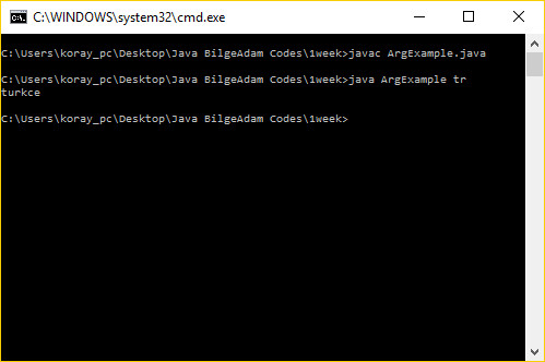
Class kodlarının içersinde ana fonksiyonumuzu public static void main olarak tanımlıyoruz. Parantezler içersinde görüldüğü gibi String[] ar...