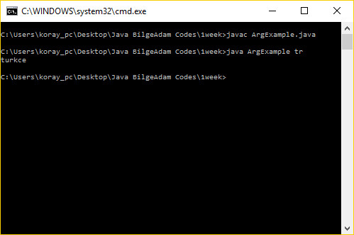
Class kodlarının içersinde ana fonksiyonumuzu public static void main olarak tanımlıyoruz. Parantezler içersinde görüldüğü gibi String[] args yazıyor. Yani ana fonksiyonumuz input olarak bir string alıyor. Terminal içersinde kod çalıştırılırken programa gerekli argümanlar gönderilebiliyoruz. Aşağıdaki örneği terminalde derledikten sonra , java ArgExample tr şeklinde çalıştırırsak args dizisinin ilk elemanu tr olduğu için program ekrana turkce yazdıracaktır.
public class ArgExample{
public static void main(String[] args){
switch(args[0]){
case "tr":
System.out.println("turkce");
break;
case "en":
System.out.println("english");
break;
case "it":
System.out.println("italiano");
break;
}
}
}

Değişkenler
Değişkenler ikiye ayrılıyor. Primitive types ve reference types olmak üzere. Referens tipleri biz tanımlayabildiğimiz için sonsuz sayıda referans tipi vardır. String bir referans tipidir. Onun dışında 8 adet primitive tip vardır. Bunlar byte , short , int , long , float , double , char , boolean
public static void main(String[] args)
{
// ***** primitive types ****
// tam sayı değişkenler
byte b=10; // 1 byte
short s=12; // 2 byte
int i = 1445; // 4 byte
long l = 123456; // 8 byte
System.out.println("byte:"+b);
System.out.println("short:"+s);
System.out.println("int:"+i);
System.out.println("long:"+l);
// kayar noktalı sayılar
float pi = 3.14f; // 4byte,f koymazsak çalışmaz.
// otomatik olarak double yapıyor.
double d = 3.14d; // 8byte
System.out.println("float:"+pi);
System.out.println("double:"+d);
// Character
char gender = 'm';
System.out.println("character:"+gender);
// Bool
boolean bool = false; // true // 1byte
System.out.println("boolean:"+bool);
// String
String firstName="Ali";
String lastName="Veli";
System.out.println(firstName+" "+lastName);
System.out.println("Bana dedi ki \n \"sen buraya gel\"");
/*int x = 10;
{
int x = 0;
System.out.println(x);
}
{
int x = 20;
System.out.println(x);
}
*/
/*
int x = 10;
int y = 20;
System.out.println(x+y);
*/
// TYPE CASTING
Türler arasında dönüştürme yapılması işlemine type casting deniliyor. Bunun için hafızada kapladığı alanı daha küçük olan değişken , daha büyük bir değişken türüne dönüştürülmelidir. Aksi takdirde veri kaybı olması ihtimali vardır.
// IMPLICITLY CASTING
// implicitly = kesin olarak , tam olarak
/*
byte bNumber = 12;
int iNumber = bNumber;
System.out.println(iNumber);
*/
// EXPLICITLY CASTING
//Veri kaybı olma ihtimali olan durumlarda
//compiler kodu derlemiyor. Derlemesi için casting
//operatörünün kullanılması gerekiyor.
int iks = 1034;
// 00000000 00000000 00000100 00001010
byte be = (byte)iks;
System.out.println(be);
int posX = 12;
float posY = posX;
System.out.println(posY);
System.out.println((int) pi);
}
}
OPERATÖRLER
public class Operators{
public static void main(String[] args)
{
// Aritmetic operators
int x = 10;
int y = 3;
System.out.println(x+y);
System.out.println(x-y);
System.out.println(x*y);
System.out.println(x/y);
System.out.println(x%y);
System.out.println(++x); // prefix postfix
/* ++ operatörü x değişkeninin önüne geldiği için ilk önce x'i bir arttırır , sonra x ile ilgili bir işlem yapılacaksa onu yapar. */
System.out.println(x--);
/* Burada x ile ilgili işlem yapılır daha sonra x bir azaltılır.
x=x+1;
x+=5; // x 5 arttırılır , yine x değişkenine atanır.
x-=5; // x 5 azaltılır , yine x değişkenine atanır.
x*=5; // x 5 ile çarpılır , yine x değişkenine atanır.
x/=5; // x 5'e bölünür , yine x değişkenine atanır.
// Bitwise operators
byte k = 10 ;
// 0000 1010
// 1111 0101
System.out.println(~k); // bitwise unary NOT
byte a = 10; // 0000 1010
byte b = 20; // 0001 0110
// 0000 0010 &
//
System.out.println(a&b); // binary AND
System.out.println(a|b); // binary OR
System.out.println(a^b); // binary XOR
byte q = 16;
System.out.println(q>>2);
System.out.println(q<<2);
// Relational Operators{
int a1 = 10;
int b1 = 20;
System.out.println(a1==b1);
System.out.println(a1!=b1);
System.out.println(a1>b1);
System.out.println(a1<b1);
System.out.println(a1>=b1);
System.out.println(a1<=b1);
// Logical Operators
System.out.println(true & false);
System.out.println(true | false);
System.out.println(true ^ false);
System.out.println(!true);
System.out.println(false && false);
System.out.println(true || false);
System.out.println(true? "true":"false"); // ternary if
/* Ternary if ifadesi yazım kolaylığı sağlamaktadır. iften pek farkı yoktur. Eğer iki koşullu bir durum varsa , kullanılması tavsiye edilebilinir. Soru işaretinden önceki ifade doğru ise true değilse false geri döndürür.
}
}
public class Boxing{
/* Object diye bir değişken var. Bu değişkenin
özelliği içersinde her türlü tipte bilgiyi tutabiliyor.
Aşağıdaki örnekte önce int tipte bir değişken ataması
yaptık , daha sonra aynı değişkene float bir değer ve
string ataması yaptık. Her seferinde değişken değeri
ekrana verildi. Program sıkıntısız çalışıyor ve bu verdiğimiz
değerleri ekrana yazıyor. Bu işleme boxing deniyor. */
public static void main(String[] args)
{
int x = 10;
Object obj = x;
System.out.println(obj);
obj = 3.14;
System.out.println(obj);
obj = "Koray Kara";
System.out.println(obj);
}
}